関税の影響を少しでも追跡するために、アメリカの輸入額予測をやってみたい。
ただ、関係する要因があまりにも多すぎるので、まずは、非常にシンプルに、輸入額のみを時系列分析と因果推論の時系列分析で学習と予測をやってみたい。
コードや進め方は、以下の2冊を主に参照させてもらっています。無茶苦茶、勉強になります。

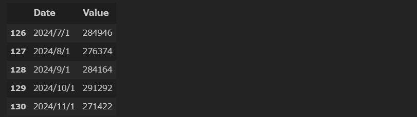
”元”データは、2014年から2024年11月までのアメリカの月次輸入額(百万ドル)。CSVファイルは以下からダウンロード可。
# ライブラリーの読み込み
from statsmodels.tsa.seasonal import STL
import pandas as pd
import warnings

warnings.filterwarnings("ignore")

# データの意味込み
df = pd.read_csv("Import.csv")

df.tail()
- 季節性をみるためにSTL分解してみる。コロナは異常値扱いできると思うが、一旦、そのままやってみる。
# STLを使って時系列を分解
# 期間は月次なので、m=12

decomposition = STL(df["Value"], period=12).fit()
import matplotlib.pyplot as plt
import numpy as np
# 各成分をプロット
fig, (ax1, ax2, ax3, ax4) = plt.subplots(nrows=4, ncols=1, sharex=True, figsize=(10,8))
ax1.plot(decomposition.observed)
ax1.set_ylabel("Observed")
ax2.plot(decomposition.trend)
ax2.set_ylabel("Trend")
ax3.plot(decomposition.seasonal)
ax3.set_ylabel("Seasonal")
ax4.plot(decomposition.resid)
ax4.set_ylabel("Residuals")
plt.xticks(np.arange(0,130,12), np.arange(2014., 2025,1).astype("int"))
fig.autofmt_xdate()
plt.tight_layout()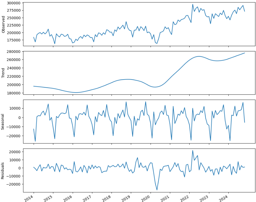
- 明確に季節性が見て取れる。
- コロナの影響で2020年の中頃に落ち込んだ後、一気に回復。トレンドとしては、コロナ以降、大きく増加傾向。
- 2022年の前半に異常値ともとれるほど上昇している。
通常の時系列分析で扱るかどうか、定常化を検査してみる(ディッキーフラー検定)。
#定常化の検査
from statsmodels.tsa.stattools import adfuller

ADF_result = adfuller(df["Value"])

print(f"ADF Stastic: {ADF_result[0]}")
print(f"p-value: {ADF_result[1]}")
- p値 > 0.05 で明らかに定常ではない。
一回差分でも定常化できそうであるが、さらに精度を上げるために2回差分でやってみる。
# 定常ではないので2階差分をとってみる
im_diff = np.diff(df["Value"], n=2)

fig, ax = plt.subplots(figsize=(10,5))

ax.plot(im_diff)
ax.set_xlabel("Time")
ax.set_ylabel("Import Value")

plt.xticks([0,12,24,36,48,60,72,84,96,108,120], ["2014","2015","2016","2017","2018","2019","2020","2021","2022","2023","2024",])

plt.tight_layout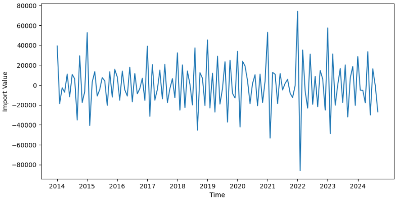
# 再度定常化の検査
ADF_result = adfuller(im_diff)

print(f"ADF Stastic: {ADF_result[0]}")
print(f"p-value: {ADF_result[1]}")
p値 < 0.05 で定常といえそう。
- 自己相関をみてみる。
# AFC
from statsmodels.graphics.tsaplots import plot_acf

plot_acf(sales_diff, lags=12)
plt.tight_layout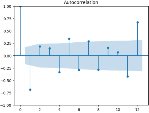
- 12ケ月毎の周期性を想定できそう。
from itertools import product

ps = range(0,13,1)
qs = range(0,13,1)
Ps = [0] # ARIMA(p,d,q)モデルを使っているのでPとQの値を0に設定
Qs = [0]

d = 2 #定常化するための差分の階数
D = 0 # ARIMA(p,d,q)モデルを使っているのでDの値を0に設定
s = 12 # statsmodelsライブラリーのsはmに相当し、どちらも頻度を表す

# (p,d,q)(0,0,0,)の組み合わせとして考えられるものをすべて生成
ARIMA_order_list = list(product(ps,qs,Ps,Qs))
# 最適なSARIMAモデルを選択する関数
from typing import Union
from tqdm import tqdm_notebook
from statsmodels.tsa.statespace.sarimax import SARIMAX
def optimize_SARIMA(endog: Union[pd.Series, list], order_list: list, d: int, D: int, s: int) -> pd.DataFrame:
results = []
# 一意なSARIMA(p,d,q)(P,D,Q)_mモデルをすべてループ処理し、それぞれのモデルを適合させ、AICの値を格納
for order in tqdm_notebook(order_list):
try:
model = SARIMAX(endog, order=(order[0], d, order[1]), seasonal_order=(order[2], D, order[3], s), simple_differencing=False).fit(disp=False)
except:
continue
aic = model.aic
results.append([order, aic])
result_df = pd.DataFrame(results)
result_df.columns = ["(p,q,P,Q)", "AIC"]
# 昇順でソート:AICの値が小さいほど良いモデル
result_df = result_df.sort_values(by="AIC", ascending=True).reset_index(drop=True)
return result_df# 訓練データセットは2023年まで(2024年はテストデータとしてみる)
train = df["Value"][:-11]
test = df["Value"][-11:]
train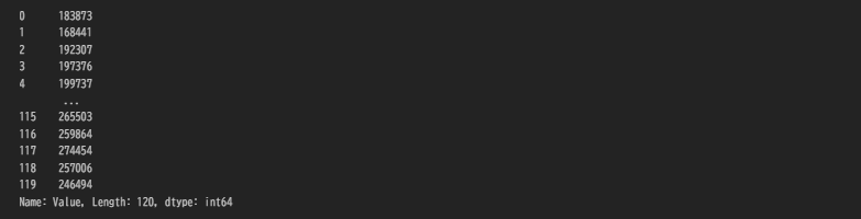
# optimize_SARIMA関数を実行
ARIMA_result_df = optimize_SARIMA(train, ARIMA_order_list, d, D, s)
ARIMA_result_df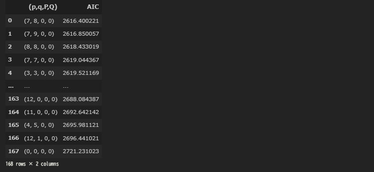
- 計算時間かかるな、、、
- AICが一番低いのはp=7、q=8という結果。
- ARIMA(7,8)でモデル化してみる。
# モデル
ARIMA_model = SARIMAX(train, order=(7,2,8), simple_differencing=False)
ARIMA_model_fit = ARIMA_model.fit(disp=False)
# 結果サマリーの表示
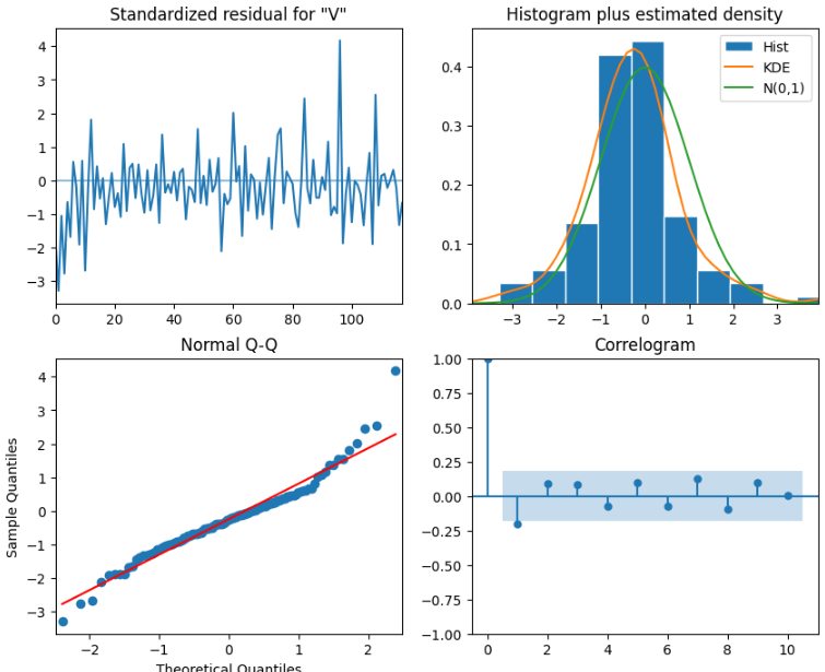
ARIMA_model_fit.plot_diagnostics(figsize=(10,8))
print(ARIMA_model_fit.summary())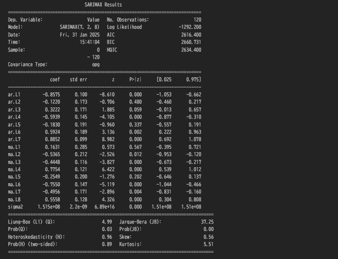
- coefのいくつかp値で0.05より上のものがあるが、おおむね0.05以下。
- 定性分析を見る限り、分散はおおむね一定、残差の分もほぼ正規分布、Q-Qプロットも両端に異常値がみられるがほぼ直線なので、使っても良さそうといえるのかな?
- リュングボックス検定で検証してみる。
from statsmodels.stats.diagnostic import acorr_ljungbox

residuals = ARIMA_model_fit.resid
result_df = acorr_ljungbox(residuals, np.arange(1,11,1))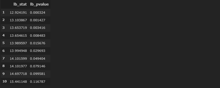
- 結果、7個で0.05以下となり帰無仮説(残差=無相関)が棄却できない。
- つまり、あてはまりのいいモデルとは言いがたい。。→ 現実は複雑なので、そもそも単純なモデルにあてはめようとすることに無理があるので、当たり前か。
- 今後の参考のために、一旦、これをこのまま進めてみる。
# 結果を格納
ARIMA_pred = ARIMA_model_fit.get_prediction(120,131).predicted_mean
test["ARIMA_pred"] = ARIMA_pred- 比較のためにSARIMAXで季節性を考慮したモデルで試してみる。
# SARIMAX
# 季節差分をとってみる
df_diff_seasonal_diff = np.diff(im_diff, n=12)

ad_fuller_result = adfuller(df_diff_seasonal_diff)
print(f"ADF Statistic: {ad_fuller_result[0]}")
print(f"p-value: {ad_fuller_result[1]}")
- p値 < 0.05なので、定常といえそう。
# p,q,P,Qに[0,1,2,3]の値を試す

ps = range(0,4,1)
qs = range(0,4,1)
Ps = range(0,4,1)
Qs = range(0,4,1)

# 次数の一意な組み合わせを作成
SARIMA_order_list = list(product(ps,qs,Ps,Qs))

d = 2 #定常化するための差分の階数
D = 1
s = 12 # statsmodelsライブラリーのsはmに相当し、どちらも頻度を表す

# optimize_SARIMA関数を実行
SARIMA_result_df = optimize_SARIMA(train, SARIMA_order_list, d, D, s)
SARIMA_result_df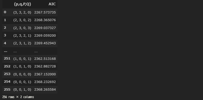
- 計算に時間かかる、、、
- AICが一番低いのは、p=3、q=3、P=2、Q=0という結果。
- これでSARIMAモデルをやってみる。
SARIMA_model = SARIMAX(train, order=(3,2,3), seasonal_order=(0,1,1,12), simple_differencing=False)
SARIMA_model_fit = SARIMA_model.fit(disp=False)


SARIMA_model_fit.plot_diagnostics(figsize=(10,8))
print(SARIMA_model_fit.summary())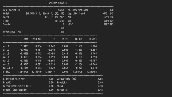
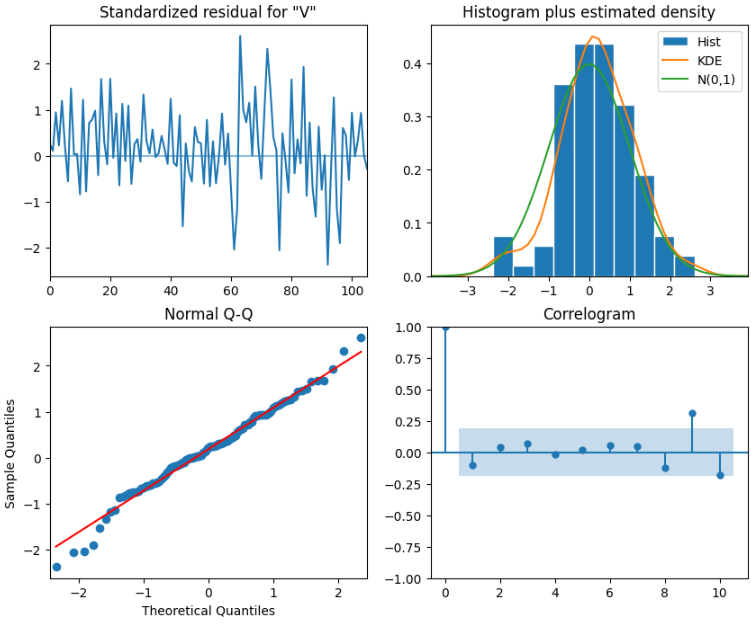
- 定性分析を見る限り、よさそうであるが、
- リュングボックス検定で検証してみる。
residuals = SARIMA_model_fit.resid
result_df = acorr_ljungbox(residuals, np.arange(1,11,1))
result_df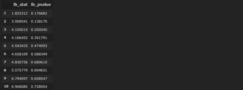
- 全てのp値が0.05より上なので、残差は無相関といえそう。
- 明らかに、先ほどのARIMAよりいい結果。
# 結果の格納
SARIMA_pred = SARIMA_model_fit.get_prediction(120,131).predicted_mean
test["SARIMA_pred"] = SARIMA_pred
# ARIMA、SARIMAXの結果の描画
fig, ax = plt.subplots()
ax.plot(df["Date"], df["Value"])
#ax.plot(test["Sales quantity"], "b", lable="actual")
#ax.plot(test["naive_seasonal"], "r", label="naive seasonal")
ax.plot(test["ARIMA_pred"], "k", label="ARIMA")
ax.plot(test["SARIMA_pred"], "g", label="SARIMA")
ax.set_xlabel("Date")
ax.set_ylabel("Import Value")
ax.axvspan(120,131, color="#808080", alpha=0.2)
ax.legend(loc=2)
ax.set_xlim(70,131)
fig.autofmt_xdate()
plt.tight_layout()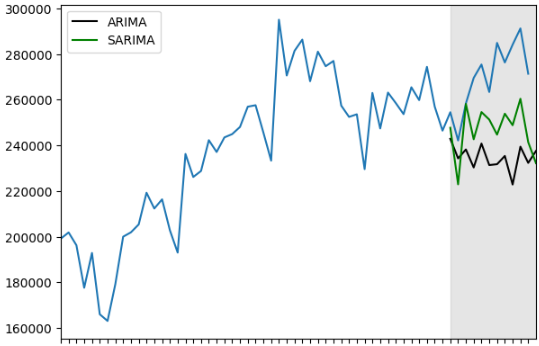
- 灰色にカラーリングした部分がtest期間(2024年)、青が現実の輸入額、黒がARIMA、緑がSARIMA
- 当たり前だが、簡単にはフィットしない。
- 明らかにSARIMAの方が現実に近いが、SARIMAでも良く予測しているとはいいがたい。
- ただ、他の見方として、モデルの予測より、現実経済の方が過熱しているともとらえられる。
- 次回は、因果推論の時系列分析でやってみる。